Rope Swing Theory

Viscoelastic Theory behind Rope Swings
with numerical solutions of the Euler Lagrange Equations
and real jumps from a bridge
1.
Viscoelastic Model of a Rope Swing |
 |
Abstract: |
| Max
Bigelmayr, Sept. 2012, March 2013 |
1.
Viscoelastic Model of a Rope Swing
1.1
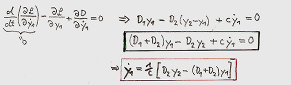
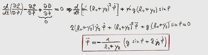
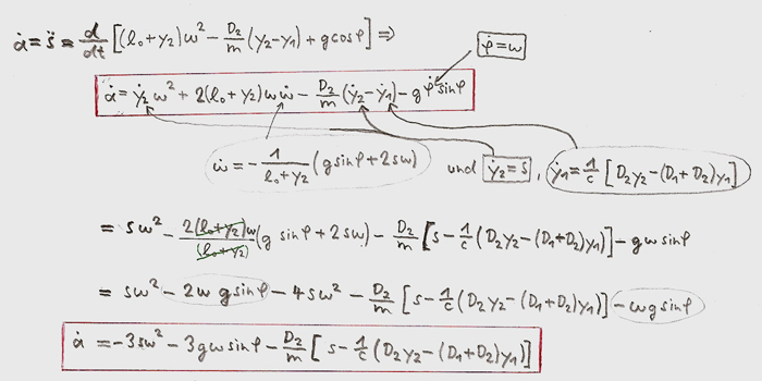
Lagrange
Equation and Dissipation Function
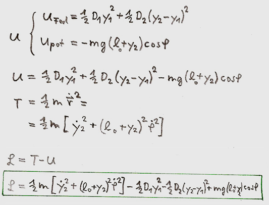
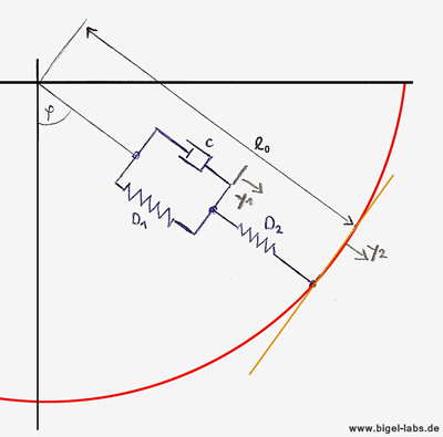
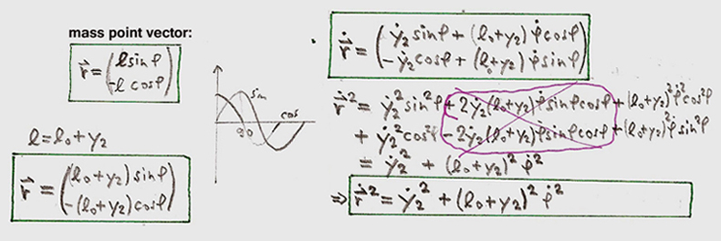
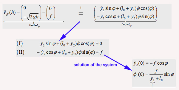
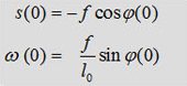
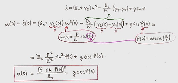
The pendulum is easily calculated with the help of Polar Coordinates. Let´s start with by discribing the mass-point, dependent on the angle P and the elongation y2. The derivation of the mass-point in realtion to time, gives us the speed vector of the mass-point as well as its absolut value squared:
|
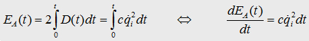
The potential energy is seperated into Spring Energy and Hight Energy. The elongation of spring 2 with the factor D2, equals the realtiv movement y2-y1: |
||
|
 |
|
| Viscoelastic
Pendulum with elongations y1 and y2
|
||
 ,
, .
. equ.(1)
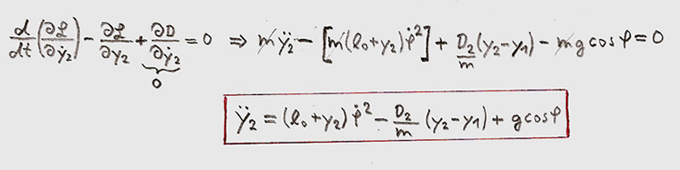 equ. (2)
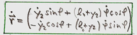
 equ.
(3)
equ.
(3)
2.
Numerical Simulations
2.1
Elasticity
moduls and typical rope-climbing parameters
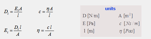
| So now let´s look at
some numerical simulations. For calculations it´s usefull to
work with lenght independent constants. |
|||||||
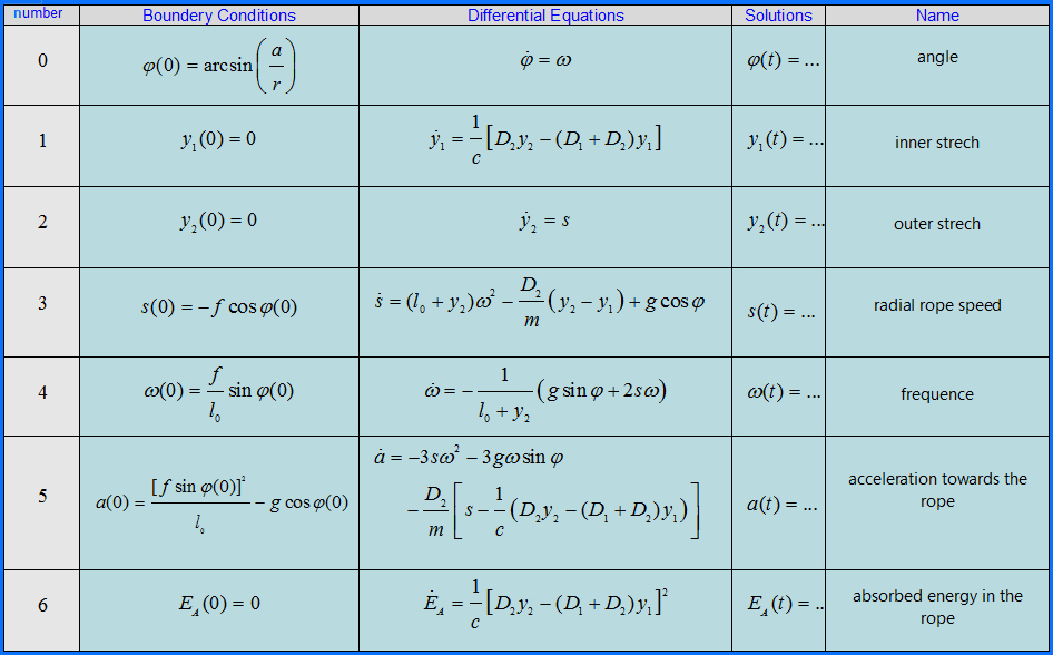
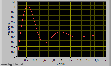
 In respect to the Viscoelastic Theory of Climbing Ropes [Ulrich Leuthäusser] one is able to discover the typical parameters of a climbing rope. These are: 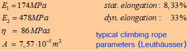 Within the Graphs on the right you are able to view the oscillations of a climber [m=80kg] falling into the rope from falling height of 5m. The curves were numerically calculated with a Cash Carp 5th order system. |
|
||||||
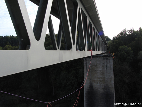
But now let´s come back to the physics behind the rope-swing.
If you´re lucky [or bad luck??? ;-)] you know a very large bridge
like this:
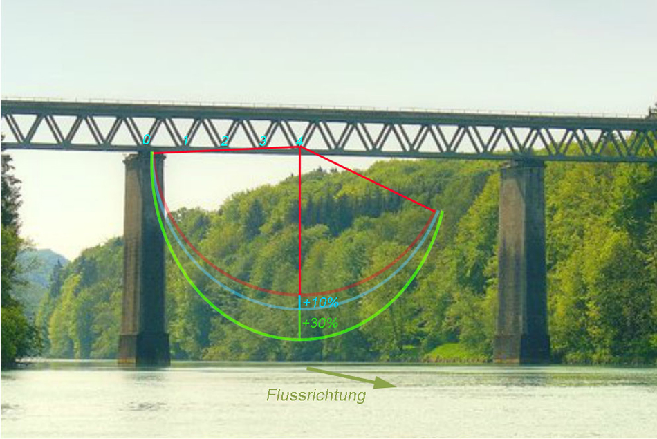
Some people enjoy falling a long way down before experiencing the ropes tension. This brings up the interesting question as to the maximum g-force that a jumper has to withstand during this stage of the rope-swing.
.2.2 Programm and numerical simulations
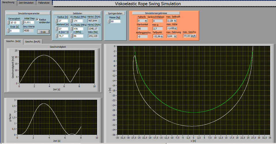
I programmed a tool with that it´s possible to analyse the fall paths in detail. All the seven differential equations may be solved by the programm numerically by a Cash Carp Algorithm. At first you have to put in the precise, simulation time, intial time step. After defining the rope parameters [lenght, cross section, elaticity modul E1, E2, constant n (Pas)] and the jumper mass you may start the simulation.
|
|
| Screenshot of the Rope Swing Simulation programm. |
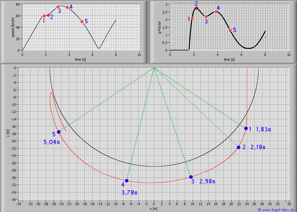
In the next step you may wath the falling paths and all the forces, speeds etc. in realtime. Annother option is to analyse specific points of the fall path in detail. [f.e. ]
The following Simulations show the paths of a 75kg person jumping with a 27m long standart climbing rope [E1=174MPa, E2=478MPa, n=86MPas, A=7,57*10^-5m^2] at different jump distances:
Jump Distance 27m 
Jump Distance 24m
Jump Distance 20m
Jump Distance 15m 
Jump Distance 10m 
Jump Distance 5m 
2.4 Analysis of characteristic points
While a rope swing the g-force maxima are interesting.
These graphs show the values for a 75kg person jumping with a 27m long
standart climbing rope [E1=174MPa, E2=478MPa,
n=86MPas, A=7,57*10^-5m^2] at a jump distance of 24m:
By analysing the maximum g-forces at certain jump distances
one gets the following distributions: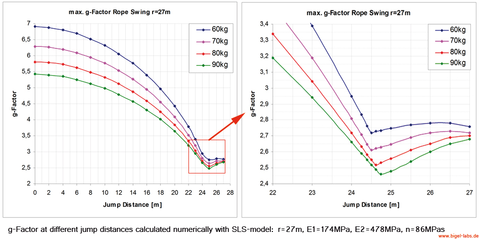
It´s quite interesting that there is a certain jump
distance beween 24m and 25m where the jumping person has
to withstand minimum g-forces during the swing.
So it´s better for dorsal to jump at around 24m.
3. Rope live-time approximation
Martyn Pavier [University of Bristol, Department of Mechanical Engineering] did some Experimental and theoretical simulation of climbing falls. He found a logaritmic dependence of the maximum tension and the number of falls to failure [graph on the right hand sight]:
|
|
| Graph1:
Numerical claculation of the maximum rope force while a rope swing
at different jump distances Graph2: Maximum tension vs. the number of falls to failure measured by Martyn Pavier |
![Rope Life Time [Rope Swing]](RopeLiveTime.jpg)
Let´s assume a rope swing jumper which has got
a jump distance of around 23-27m while his jumps[rope lenght 27m].
As Graph1 shows the maximum rope force while the
swinging is around 2kN. Comparison of this value with the number of
fails M. Pavier found one may assume that a standart climbing rope
will fail after 50-80 jumps.
Depending on the "history" of the rope the number of jumps
to failure may also be even less than 50 jumps. So it is allways
a must to use a redundance rope!
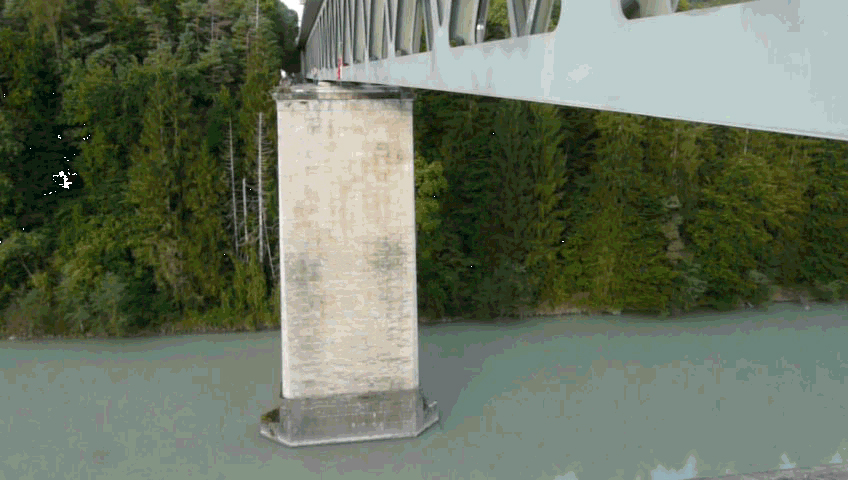
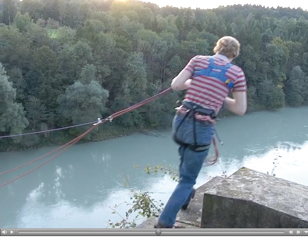
After the simulations it´s time for real jumps. We had the luck to found a 36m hight bridge...
 |
|
| Three rope system. | Preparing of the "Anker point" 36m above the ground |
 |
|
| First jump of my friend Markus [click here to watch the gif.] | |
|
|
|
| AVI-Film of my first jump [you may watch with "click".. ] | |

The
calculations and simulations which are presented here are a usefull
to get a first approximation of the forces a rope swing jumper has to
withstand during the swing.
Air resistance and rope mass are not respected in the simulations yet.
Next steps will include:
- Finding the differential equations including air resistance effects
- Multi Rope Analysis
- Static Rope Analysis
- Rope Failure Simulations [redundance rope behavior after
a failure of the main rope]
- Experimental studies and fall experiments with steel mass
falling into climbing ropes to get the exact rope parameters
So there is a lot to do....;-)

Last update: March 2013