Rope Swing- Climbing Rope Tests

Climbing Rope Stretch and Fall Tests
experiments to understand the viscoelastic behavior
1.
Viscoelastic theory of climbing ropes |
 |
|
Abstract: On this page I want to find out the specific parameters which are essential to describe a climbing rope with viscoelastic models. At first the Harmonic Oscillator Model will be described and compared to the Solid Linear State Model of a climbing rope. This model will be modified to consider the free flight of the fall mass when it bounces back. Experiments were made with one of the securest climbing ropes worldwide: The Rope "Apollo" from the manufactor Beal. Stretch tests with a 4t crane from ABUS were made to measure the hysteresis of the rope as well as fall tests with a 80kg fall mass and high speed filming of the experiments. The analysis of the fall data enabled to find typical average rope parameters for the climbing rope Apollo 11, which may be used for simulating climbing rope falls or rope swings in future. |
|
|
Max
Bigelmayr, Sept. 2013, April 2014 (V31) |
||||
1.
Viscoelastic theory of climbing ropes
1.1
Harmonic Oscillator Model (HO)
In physics nearly everything starts with the harmonic oscillator. A climbing rope may be described very easy by the harmonic oscillator. In mechanics the harmonic oscillator
contains only a simple spring with the spring constant k and a mass m.
The Lagrange equation of the system shown in [Fig. 1]
is the difference between the kinetic energy T and the potential energy U: |
 |
|
| Fig. 1: Hamonic Oscillator modell with spring constant k to describe a climbing rope fall experiment | ||
 |
||
| Fig. 2: Phases of the Hamonic Oscillator modell describing a climbing rope fall experiment: The simulation shows a rope with: E=174MPa, l=2,60m, fall height= 2,60m, m=80kg, A=95mm^2. Above the "sero line" the path of the fall mass describes a parabolic curve. |
 . [1.1]

One may seperate three phases of a fall experiment in the harmonic oscillator model: Before the stretching of the spring k the mass will be accelerated with g=9.81m/s^2 (phase 1). The start speed vo in [1.2] is the speed of the fall mass after falling down the lenght lo:
![]()
The second phase is described by [1.2] and includes the time intervall when the spring is stretched by deceleration and acceleration of the fall mass m.
While the third phase the mass is flying upwards without stretching the rope. Equ. [1.3] summarises the equations of these three phases:
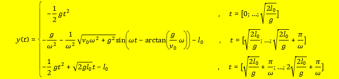 [1.3]
[1.3]
1.2
Solid Linear State Model (SLS)
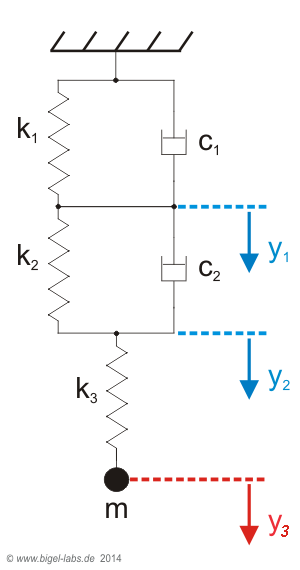
In solid state physics different methods were developed to model the behavior of viscoelastic materials. The most famous models are the Maxwell Model, the Kelvin-Voigt Model and the Wiechert Model [1]. These models use different combinations of springs and damping elements as the viscosity element n. Pavier [3] used a special SLS-model [which is called Zener k-body] to describe the stretch and damping behavior of climbing ropes during the fall of a mass m. The Zener k-body [Figure 3] contains 3 parts: Sping k1 is connected parallel to a viscosity element c1. This so called Kelvin-Voigt Model is in series with a second spring k2 with a mass m on the bottom end. The kinetic term of the system is |
|||||||||||||||||||||||||
|
![SLS-model [Zener k- Körper]](SLS.png) |
||||||||||||||||||||||||
Fig. 3.: Zener k -body as a model to describe a fall into a climbing rope. The spring k1 is parallel to the viscosity element c1. The elongation y1 is invisible and only a theoretical construct, but important to describe the energy dissipation of the system. The elongation of spring k2 is represented by y2, which is the movement of the fall body with mass m. |
|||||||||||||||||||||||||
Such a 3th order Differential equation may be solved numerically by mathematica, matlab, labview etc. by defining a differential equation system:
Table 1: Differential equations of the SLS model of a climbing rope with |
|||||||||||||||||||||||||
1.3 Comparison between HO and
SLS-Model
Booklets about climbing ropes and security advices often present the harmonic oscillator as "physical background knowledge". Based on the "Standart Equation of Impact Force" [9] some people try to calculate the forces of climbing ropes with the harmonic oscillator model. In this model the climbing rope is only described by the modulus of elasticity, the lenght and it´s cross section. With the harmonic oscillator model it´s in generall not possible to fit the impact force given by the manufactor together with the dynamic elongation. Whenever you found a perfect value for the modulus of elasticity to fit the maximum imopact force, the dynamic elongation does not fit well. If the dynamic elongation is well described the impact force is wrong. As shown in fig. 2 the harmonic oscillator system may not absorb energy, so that the fall mass will be accelerated back to it´s original start height. It´s obvious that this does not happen in real. Leuthäusser overcame this problem by fitting the data of many different climbing ropes [4] with the SLS model of a climbing rope. In his work he provided typical values for a standart climbing rope as E1=174MPa, E2=478MPa, n=86MPas, A=75mm^2. |
|
1.4 SLS-Model with loops at the climbing rope ends
In practise a climbing rope is used with two loops at the endings(fig. 6a). In general the loops are kinked with a figure eight knot or the yosemite bowline knot. In fall experiments it´s also necessary to create loops at the endings to fix on end of the rope at the ceiling. At the other end of the rope the fall mass is fixed. Le´ts assume a climbing rope with a lenght lo of 300cm between the knots. The lenght of the loops s1 (when they are elongated) are typical around 20cm (distance from the knot to the loop end). In this case the two fix points of the rope have got a distance of 340cm. Then, around 88% oft the rope is a single rope, while 12% of the rope is a dopple rope created by the loops. So in a theoretical describtion of climbing ropes it´s essential to consider "these 12% loop-endings". In fig. 6a you see the schematic diagramm of the loop model (model1). In a next step we may combine the two ropes of each loop to one "double rope" (model 2). Then model 2 may be redistributed, so that we get finaly the simulation model (fig. 6b).
The simulation model (fig 4b) may be described by a differential equation system very easy without finding six differential equations for all the hights y1, y2, y3, y4, y5, y6 you would require in the model presented in fig. 6a. But before finding the differential equations let´s think about the new parameters k1´, k2´, k3´, c1´ and c2´:
After defining the parameters we may find the differential equations to describe the "simulation model". Instead of k1´, k2´ etc. let´s omit the strokes henceforth: Differential Equations of the loop model |
|||||||||||||||||||||||||||||||
The kinetic term of the system is:
|
 |
||||||||||||||||||||||||||||||
| Fig. 7: Viscoelastic Model of a climbing rope with loops on both ends | |||||||||||||||||||||||||||||||
| The parameters in fig. 5 may be calculated by these formula: Note that EI is the elasticity modul of the climbing rope, which is parallel to the viscosity (equal to k1 in Zener k -body, Fig. 3). EII is the elasticity modul in series with the spring k2. As explained before the strokes are omited in the differential equations on the left (k1´--> k1 etc.). |
|||||||||||||||||||||||||||||||
As you see the equation (4.1) has got the differential dy2/dt in the term, equation (4.2) includes the term dy2/dt. In a differential equation system these differentials have to be substituted. Elimination of dy2/dt in (4.1) and (4.2) gives the follwing differential equation system: |
|||||||||||||||||||||||||||||||
Table 2: Differential equations of a climbing rope with loops on both ends. |
|||||||||||||||||||||||||||||||


2.
Stretch Tests with Beal Rope "Apollo"
2.1 Setup of the Stretch Experiments
While this project I was specially interested in the parameters k1, k2 and c [Fig. 3] of the climbing rope Apollo II from the manufactor Beal. This rope is one of the worlds strongest multi fall climbing ropes. Beal gives the following the informations about the rope: |
|||||||||||||||||||||||||||||
|
 |
||||||||||||||||||||||||||||
| Table 1: Datas about the Climbing Rope Apollo II from the manufactor Beal | Fig. 8: Beal Rope Apollo II, 50m, d=11mm | ||||||||||||||||||||||||||||
| In the following tests a brand new climbing rope was used [Fig. 6] to find the wanted parameters. At first the parameters k1 and k2 has to be found. But sadly it´s not possible to find the exact values of k1 and k2 directly by stretching the rope. If you stretch the rope very slowly the viscosity c may be neglected. In this special case the Zener k-body becomes a simple setup with the two springs k1 and k2 in series. The spring rate then is The value of K may be measured by a climbing rope strech test: |
|||||||||||||||||||||||||||||
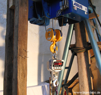
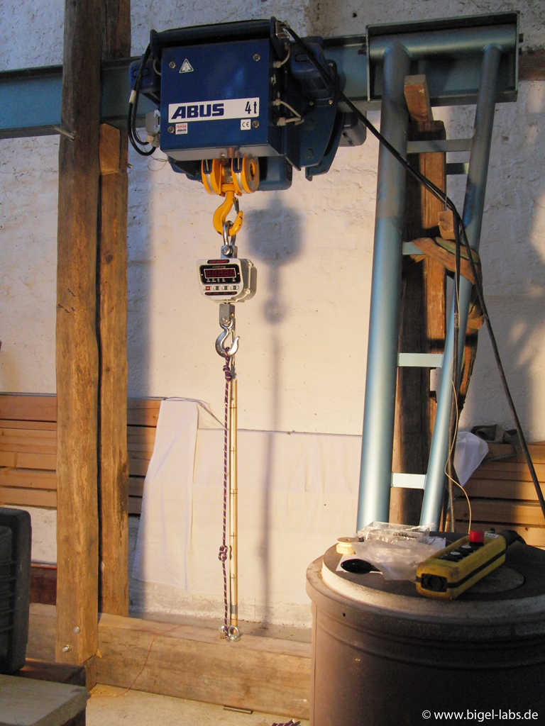
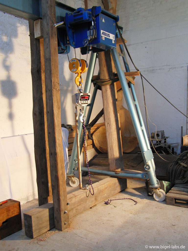
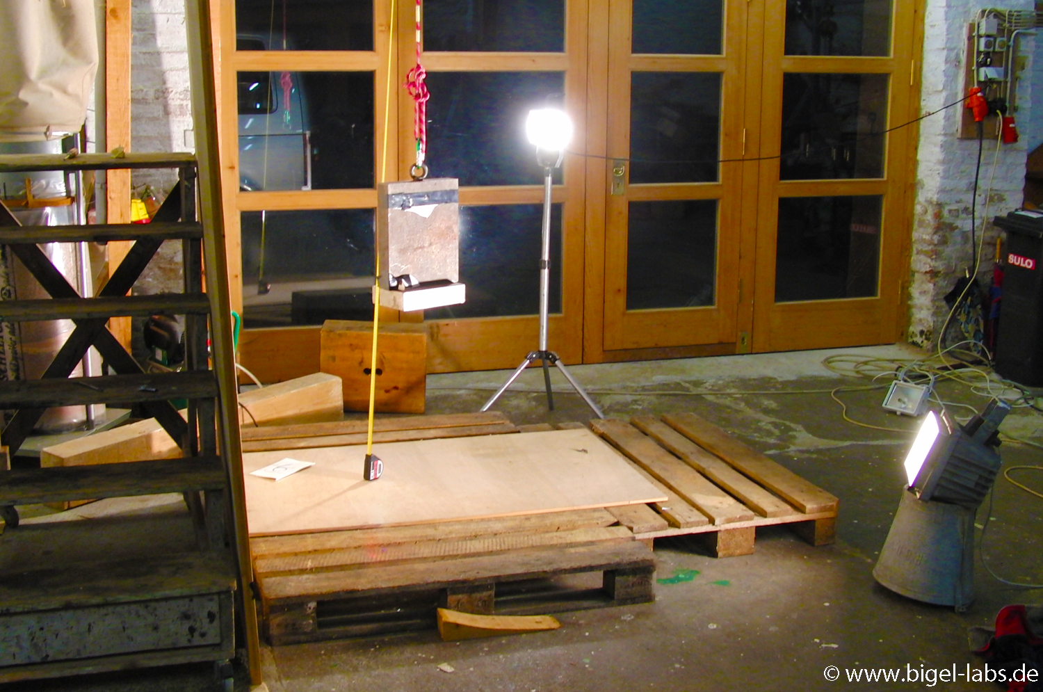
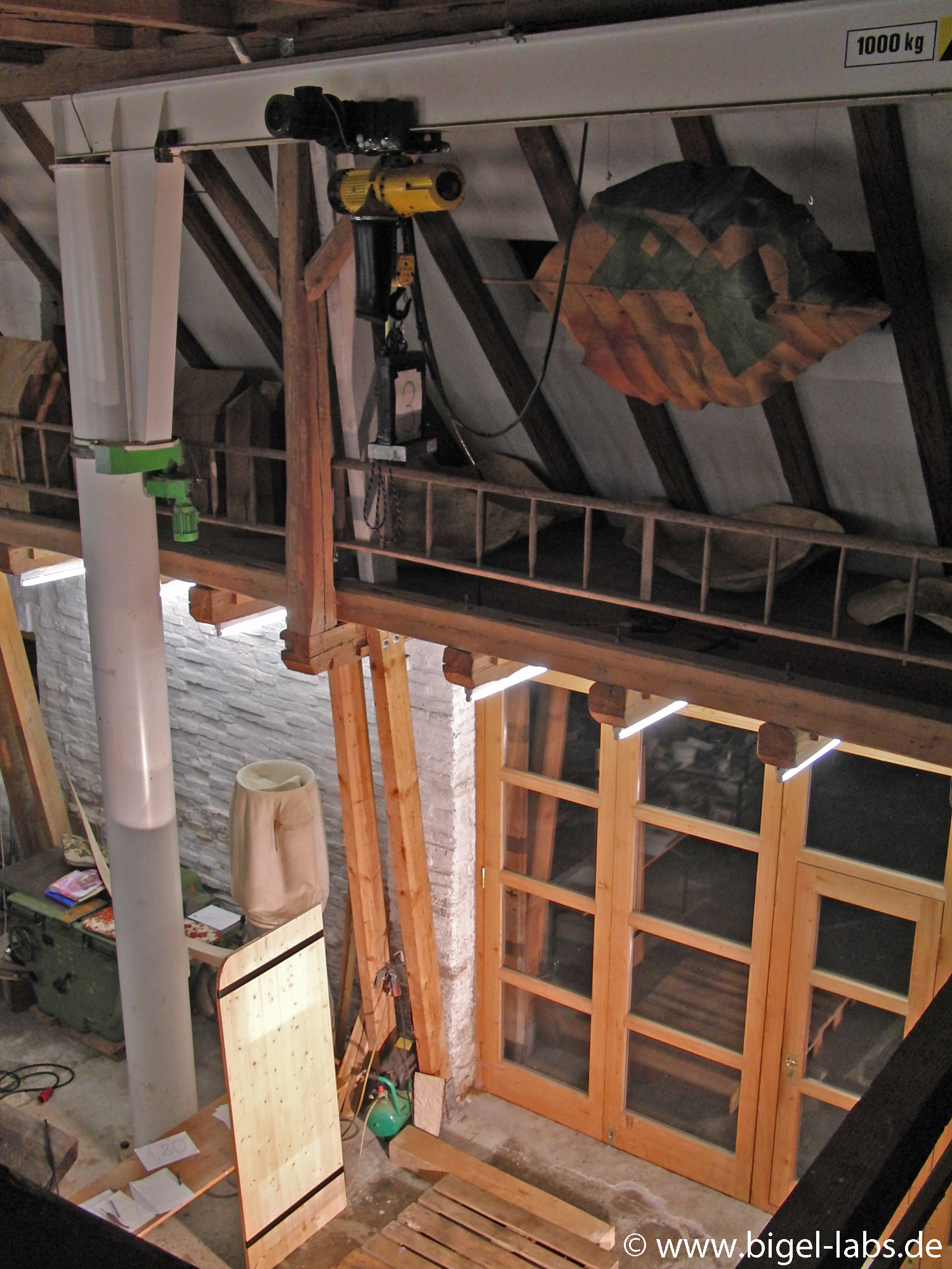
To find the parameter K a large 4 tone crane from Abus was used. Sadly we haven´t got any wight which is heavier than 2000kg. Therefore it was necesarry to constructed a special strech setup with woodn beams and threaded rods. Together with a friend we builded the following testing bench:
 |
 |
 |
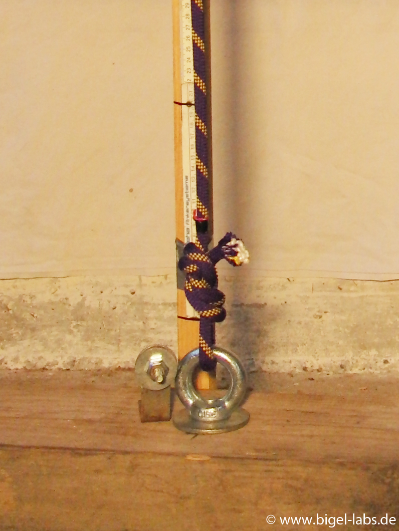 |
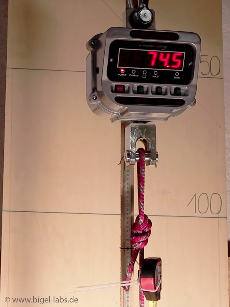
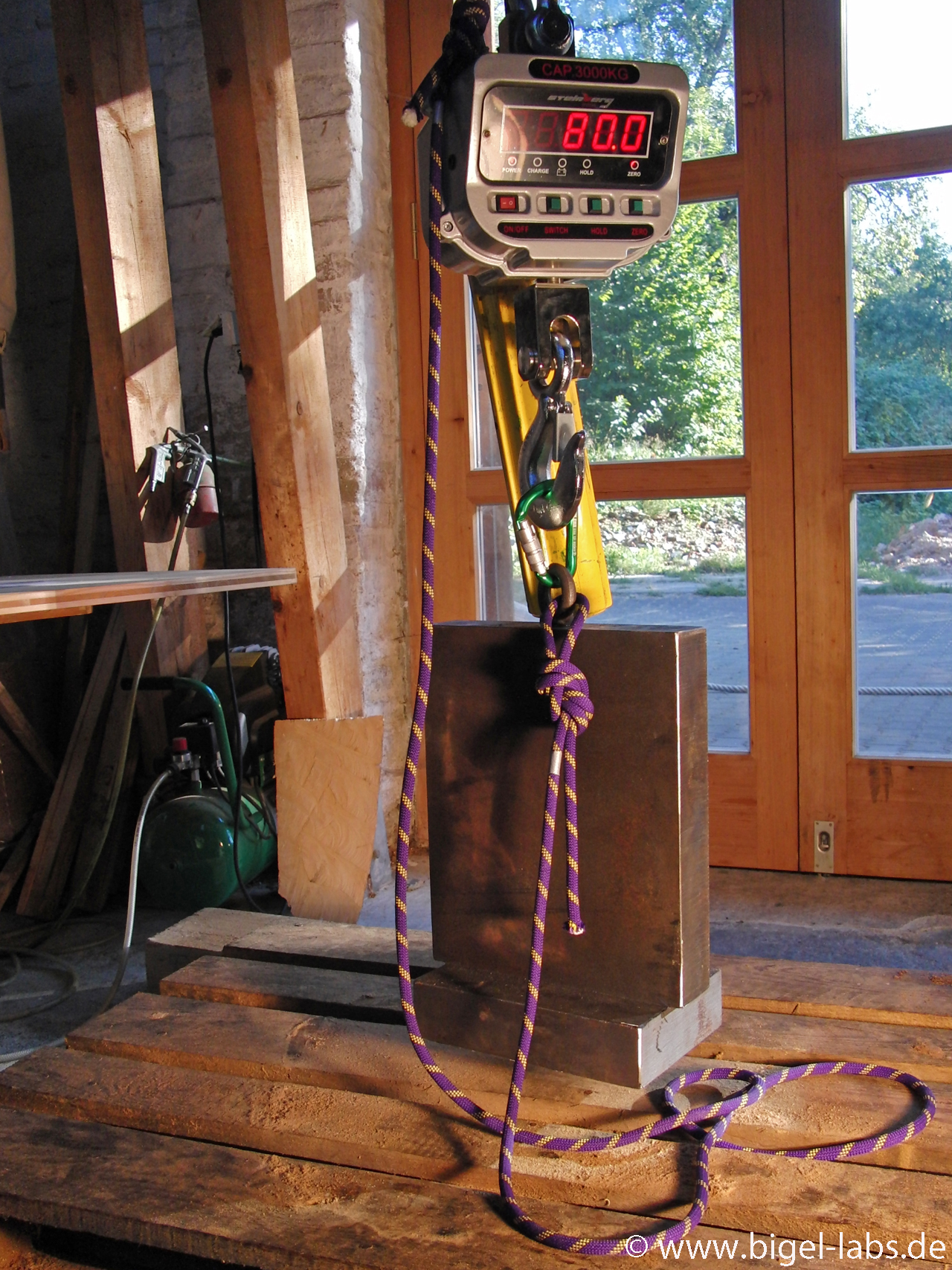
| Fig. 9a: climbing rope testing bench | Fig. 9b: climbing rope testing bench | Fig. 9c: 3000 kg crane scale | Fig. 9d: bottom hook with climbing rope |
While a test a piece of climbing rope is cutted to a lenght around 3m. On both ends figure-eight loops will be done. One loop of the rope will be thread into the hook of the beam on the floor, the other loop will be thread into the hook of the weighing scale from steinberg systems.
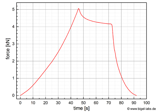
2.3 Exponential Decay of Force
While the experiment the crane drags the rope at a constant speed upwards. Thus the
force is created because of a certain lenght, the crane defines.
So the force is a function of l, as well as a function of the
time t. In the graph on the right one may watch the the force F depending
on the time t [F=9.81N/kg*m]. When the engine of the crane is
stopped at 46s the lenght of the rope does not change. But the
scale shows a decaying of the force in the rope while the time
space t=[46s,...;72s]. I tried to find a fit function for this intervall. |
 |
|
Fig. 10: Force at the rope in dependence of the time.
In the first 46 seconds the force is growing up nearly linear.
In t=[46s,...,72s] the engine of the cran is off. In this time
the force decays exponential (Fig. 7). After
72 seconds the force is reduced again by driving the crane hook
back again. |
||
|
||
2.4 Quasistatic Modulus of Elasticity In Figure 7 I made two different fits to find the derivation of the force to the lenght of the rope, which is equal to the spring rate K of the rope: |
|||||
|
 |
||||
| Fig. 12: Hyperbolic relation between E1 and E2 to fit Emin and Emax |
|||||
|
|||||


 [3.1]
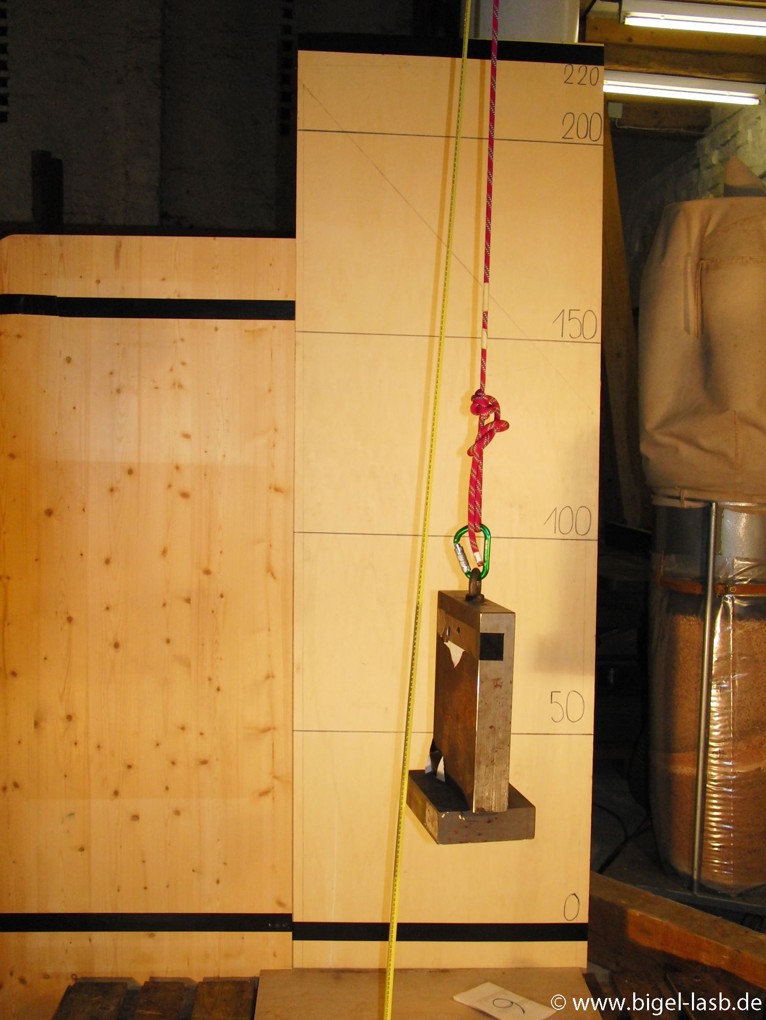
[3.1]| 3. Fall Tests with Beal Rope "Apollo" 3.1 Setup of the Fall Experiments With the stretch experiments I measured the quasi static behavior of the climbing ropes. To understand the real dynamic bahavior I build a special fall test setup for filming the fall movement with a high speed camera:
3.2
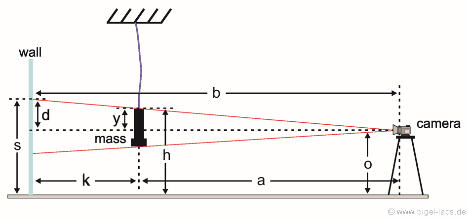
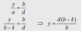
Geometry at High Speed Filming |
||||||||||||||||||
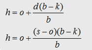
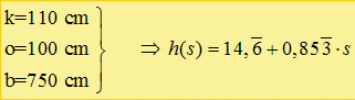
With
equation [6.1] it´s easy
to calculate the real hight of the fall mass out of the high speed films. You have just to put in the admittance s To check out the accuracy of this correction term for practical purpose I made "a small experiment" first:
3.3
Position Measurement Programms
Fall Experiment 1 Fall Experiment 2 Fall Experiment 3 Fall Experiment 4 Fall Experiment 5 Fall Experiment 6
|
||||||||||||||||||
 [6.1]
[6.1]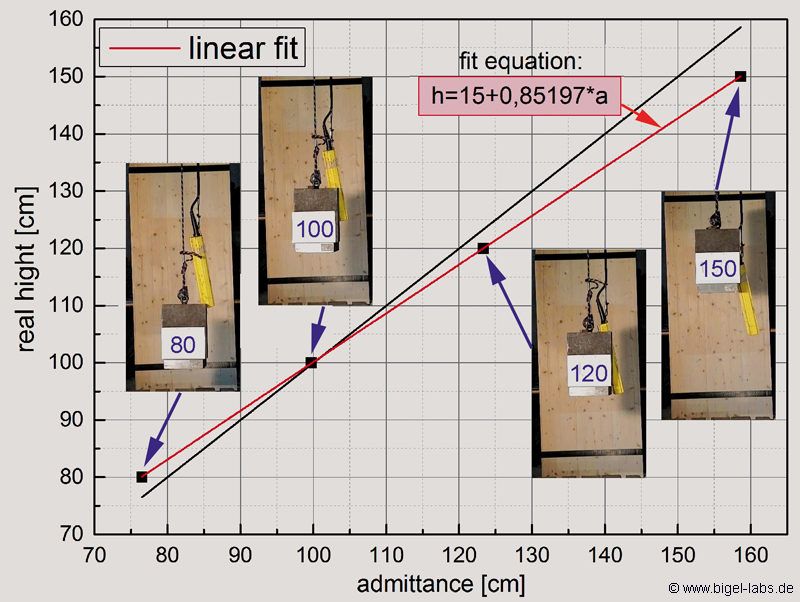
 [6.2]
[6.2]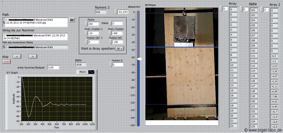
4. Fit program for Analysing the Fall Experiments (SLS-Model with loops at the climbing rope ends)
After measuring the data (presented in chapter 3.4) the curves had to be corrected geometrically by a correction term described in chapter 3.3. In the experiments with the Beal Climbing rope the correction Term was h(a)=11,57+0,914*a. With this correction the follwing Graph was obtained: |
 |
 |
| Fig. 19a: Elongation of the fall mass while the third fall experiments. The red line shows the measured data captured via the measurement programm. The blue line is corrected by the geometric correction term h(a)=11,57+0,914*a. The difference between the two curves proves the necessity of the correction process. |
Fig. 19b: Heights of the fall mass. The curves were captured via the Measurement Programm and geometrically corrected with a specific correction formula. Depending on the fall number the fall body stretches the climbing rope moore and moore. Increasing the fall numbers means a larger magnitude of the turning points. The red dashed lines are the ending values of the oscillations. |
These corrected position graphs do represent the experimental results of the SLS-model with loops at the end of a climbing roope I described in chapter 1.4.In Table 2 I showed the differential equations, which have to be solved numerically. By Variing the parameters k1, k2 and k3 it´s possible to find the ideal combination to get curves, which fit the measured lines shown in Fig. 21. To handle this fit process I programmed a special Labview VI for changing the parameters to find the ideal model parameters E1 E2 and n: |
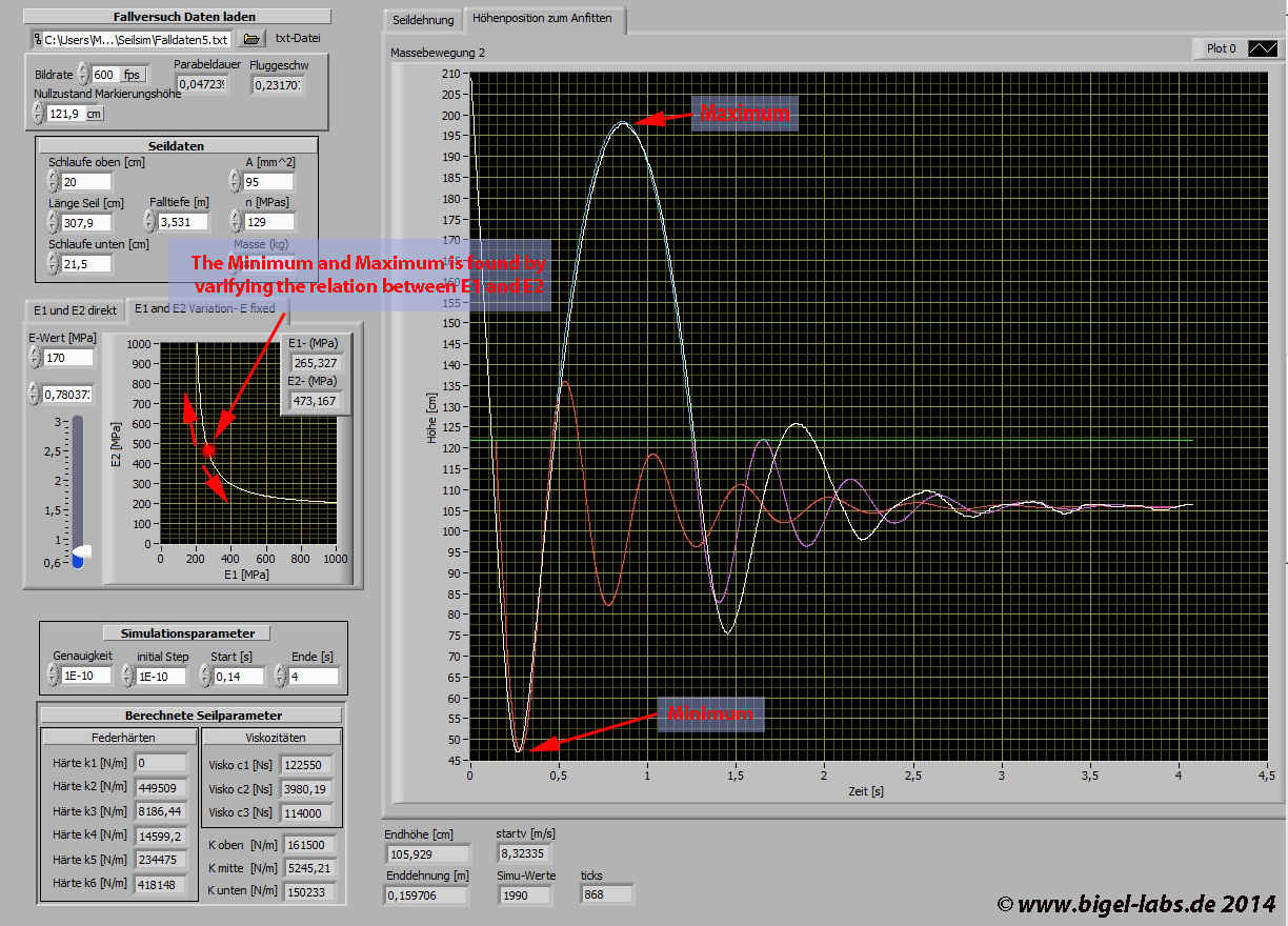
Fig. 20: Fit program for numerical simulation of the differential equation system presented in table 2. The measured experimental data (txt-file) may be loaded into the program. Then the specific values of the experiment (table 3) have to be typed in (Seildaten in fig. 22) After defining a certain accuracy (nomally I use 1E-10) the differential equation system will be solved numerically by a Cash Carp 5th order method. The variation of the relation between E1 and E2 on the hyberbolic curve (remember equation [3.1], fig. 10) and the viscosity modul gives the optimal curve. The "tension line" in green is the hight where the rope begins to be stretched while the fall process. Therefore the value of the "tension line" is equivalent the the hight, where the free fall ends. When the body accellerates back towards the maximum the simulation of the differential euquation system is interuppted at the tension line. Then the trajectory is described by standart parabolic equation (school physics). The boundary condtions at the tension line have to be equal for the differential equation and the parabolic curve to get a smooth curve. After reaching the tension line again at around 1,25s the differential equation system uses again the boundary conditions of the parabolic curve as initial conditions for the next simulation segment. The red line shows the simulation result without segmented simulation. |
5.
Fitings of the Fall Datas
5.1
Fit data with rope lenghts
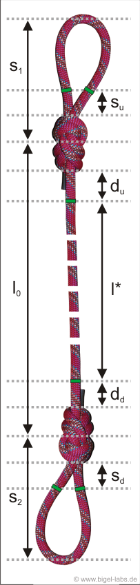
| The climbing rope I used in the fall experiments may be seperated into three parts (Fig. 22): The upper loop with the lenght s1, the middle part rope lo and the down loop s2. All these lenghts do depend on the fall number: |
| Fall Number | lenght loop s1 [cm] |
lenght loop s2 [cm] |
lenght rope without wight [cm] |
lenght rope with wight [80kg] after exp. [cm] | hight above ground after exp. [cm] |
rope lengt with loops [cm] | tension line [cm] | fall deep [cm] | fall factor |
1 |
17,2 |
18,7 |
294,7 |
310,2 |
122,5 |
346,1 |
141,4 |
333,6 |
0,96 |
2 |
19,6 |
21,1 |
300,1 |
315,9 |
115,3 |
356,6 |
130,9 |
344,1 |
0,96 |
3 |
19,8 |
21,3 |
303,6 |
319,6 |
111,4 |
360,7 |
126,8 |
348,2 |
0,97 |
4 |
19,9 |
21,4 |
307,1 |
323,3 |
108,3 |
364,6 |
122,9 |
352,1 |
0,97 |
5 |
20,0 |
21,5 |
307,9 |
324,1 |
105,9 |
365,6 |
121,9 |
353,1 |
0,97 |
6 |
20,0 |
21,5 |
309,1 |
325,4 |
104,3 |
366,9 |
120,6 |
354,4 |
0,97 |
Table 3: Length values depending on the fall number. The lengths were measured after every fall event. The values "lenght rope without wight" are not measured. I assumed that the values "lenght rope without wight" are 95% of the "lenght rope with wight aftter exp.". 95% is the typical elongation of the Beal rope without fall body compared to the lenght with the 80kg fall body I measured with the Beal rope before starting the fall experiments. In all experiments the upper ending of the climbing rope has got a hight of 495cm, while the hight of the fall body above the ground was 475cm. The fall body is allway 7,5cm lower than
the down end of the climbing rope because of the carabiner (compare fig. 11b). |
 |
 |
|
Fig. 21b: Distance between marks and knots. The distance at the upper knot is du, the distance at the bottom knot is dd. Before the first fall the distance was 0cm. After the 4th. and 5th. fall experiment I made some measurement failures, which were corrected afterwards (dashed red line). |
||
 |
||
| Fig. 21a: Rope and loop lenghts. While the experiments all lenghts in this figure are growing up. |
Fig. 21c: Rope lenght l* depending on the fall number. After each fall eperiment the rope lenght l* is growing up. I am not sure whether there is a "quasi asymtotic" behavior or not. The rope lenght where measured between the marks (Fig. 22a) while the 80kg fall mass is hanging on the rope. |
| Sadly I did not measured the lenghts s1 and s2 while the fall experiments. Therefore I assumed that the distance behavior is su=1/2du and sd=172dd. The lenghts s1 and s2 may be assumed by analyzing Fig. 22a. Let´s assume that the differential stretching per lenght d"strech"/ds after each individual fall is allways 50% of the strechting we see in Fig. 22c, because of the dopple rope inside the loops. Fig. 23a shows the assumed stretch behavior of the distances su and sd. |
 |
 |
| Fig. 22a: Assumed lenght of the loop rope parts drawn out of the knots sd and su. The lenghts are the half values of the average lenghts in Fig. 22b. | Fig. 22b: Lenght of the loops s1, s2 without 80kg mass depending on the fall number. The values are calculated and assumed with the known end value after 6 falls. |
 |
 |
| Fig. 23a: Data fit of Fall experiment 1 |
Fig. 23b: Data fit of Fall experiment 2 |
 |
 |
| Fig. 23c: Data fit of Fall experiment 3 | Fig. 23d: Data fit of Fall experiment 4 |
 |
 |
| Fig. 23e: Data fit of Fall experiment 5 |
Fig. 23f: Data fit of Fall experiment 6 |
The found fit parameters are different for any individual fall experiment. In fig. 25a and Fig. 25b the found parameters are shown
as a function of the fall number:
 |
 |
| Fig. 24a: Fit parameters for the first positive and negative peak (Fit 1) | Fig. 24b: Fit parameters for the second positive and second negative peak (Fit 2) |
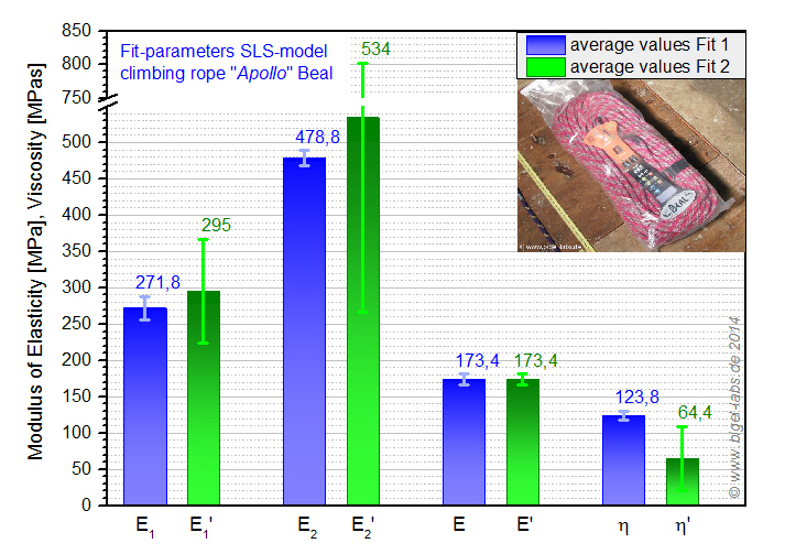
| Averages of the fit parameters (fall 2-fall 6) are presented in fig. 26. The average values Fit 1 are usefull for further simulations (rope swings etc.) with the climbing rope "Apollo". Fit 2 is not that suitable for simulations because of it´s large standart derivations. |
 |
|
| Average Values E1= 272MPa E2= 479MPa n = 124MPas |
Fig. 25: Averages of the fit parameters of the climbing rope Apollo from Beal . The values from the 2.-6. fall are averaged. E1, E2, E, n are the fit parameters of the SLS-model for the first negative and positve peak of the fall curves. E1', E2', E', n' are the fit parameters of the SLS-model for the second negative and positive peak of the fall curves. The values E1', E2', E', n' are not that usefull because of it´s large standart derivations. |
| In this work I first decribed the harmonic oscillator model for a climbing rope drop test. Based on the problems to find perfect parameters to describe the impact force together with the dynamic elongation of the rope the solid linear state model for a climbing rope (SLS-model) was presented. The typical SLS-model for a climbing rope was supplemented with a description of the loops at the ends of the climbing rope. In the experimental part climbing ropes where streched with a self built testing bench. With a crane (and crane scale) the climbing rope Apollo from the manufactor Beal was stretched and the hysteresis curve was measured up to an accuracy of +-0,5kg and appr. 2mm. On the basis of the gradient the modulus of elasticity was evaluated to a value of E(min)=136MPa, E(max)=158MPa. Futhermoore the exponential decay of the force at the climbing rope stretched to a fixed lenght was analyzed. It was shown that the decay of the force may be described quit well by a double exponential function. |
| Fall experiments were made with a 80kg falling weight to find the parameters E1, E2 and n of the SLS-model. Therefor the falling weight was droped down appr. 3,50m into the Apollo rope six times by a fall factor of appr.1 to analyse the elongation and damping process. The movement of the weight was filmed by the high speed camera Casio Exilim F1 at a frame rate of 600fps at a resolution of 432px*192px. Afterwards the exact values of the fall paths were captured by the Lucas Kanade algorithm for each individual frame. The recorded data were corrected geometrically by a specific correction term which is appropriate to the experimental scales in the experimental setup. | 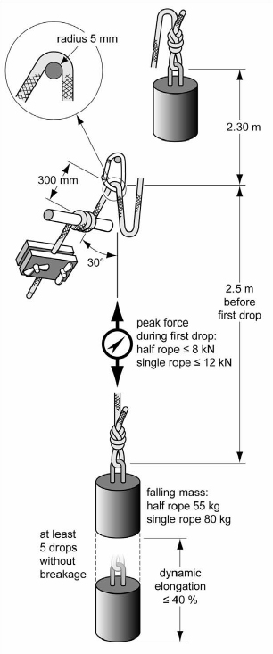 |
||
A comparison of the different fall paths according to the six fall experiments gave a continuous decrease of the height of the turning point (maximum elongation). Each further drop test gave a larger elongation value than the drop test before as well as a higher vertex of the parabola after the phase when the fall weight bounces back (fig. 19b). The end hights after each individual fall tests do also lower from fall to fall. Associated the with this the rope lenght (between the loops) itself increases approx. up to 4% if you compare the lenght after the 6th fall with the lenght after the 1th fall (fig. 21c). While the 1th fall the damping of the oscillation process is dominated by tighting up the figure eight knots at the loops. This effect causes a relativ large difference oft he height curve hfall 1-hfall 2 in comparison to the other differences hfall3-hfall2 etc. (fig. 19b, 21b, 22a,b). |
|||
Analyses of the measured oscillations were made with a self built "Fit program", which uses the differential equation system (ODE= Ordinary Differential Equations) for climbing ropes with loops at the ends presented in capter 1.4. The ODE was solved numerically with a Cash Karp algorithm of 5th order for different values for the parameters E1, E2 and n. With adaptive variation of the parameter values I could found individual "sets of E1, E2,, n) for each fall experiment (fig. 23a-f). It was shown that it´s not possible to find such a parameter set describing the entire oscillation process while one drop test. Hence it seemed to be practical to subdivide the fits into two splines with smooth boundary conditions at the endings. The first splines (in blue ) are suitable to desribe the first negative peak and to maximum of the parabloic flight, while the second splines (in green) do fit the swing off in fig. 23a-f. |
|||
The average of the fit parameters (first spline fit fall 2-6) was calculated so that I got the follwing values for the climbing rope Apollo:
These values seem to be quit good for fall factors [0,..,1]. Simulations for larger fall factors like 1.7, (which is used in the standart drop test by the UIAA (fig. 26)) do varify in comparison to the data given by the manufactor Beal (table 1). |
|||
| Fig. 26: Standart Drop Test geometry (source [8]) | |||
The experiments do suggest the assumption that the values E1, E2,, n one may get by analysing the fall experiments do depend on the fall factor used in the experiments. Whenever you try to find the fit parameters E1, E2,, n for a specific climbing rope on the basis of the datasheets by the UIAA drop tests, you will find many different sets of E1, E2,, n which fit the impact force, dynamic elongation and end elongation. In my opinion it´s necessary to fit the entire osciallation process with respect to the maximum parabolic flight height, as I did in this publication. Another point is the 300mm path before the carabiner in the standart drop test (fig. 26). This rope section grates at the carabiner, which qualifies a new model including energy dissipation effects when using the UIAA drop tests data to find the parameters of a climbing rope in the SLS model. Assigning the results of the experiments of this publication to the physics of rope swings I made path simulations with all found fit parameters from fig. 25a, b. All paths of the six simulations are higher than the path of a typical climbing rope from Leuthäusser [4] with E1= 174MPa, E2= 478MPa, n= 86MPas, A=75mm^2. The rope swing path with the found average parameters from the climbing rope Apollo with E1= 272MPa, E2= 479MPa, n=124 MPas, A=95mm^2 is marked green in the following graph: |
Fig. 27:
Swing paths of a
rope swing simulated with the found fit parameters. The
upper blue line is the radius of the rope (27m), the down line in red
represents the swing with a typical climbing rope, with the parameters
found by Leutheusser. Rolling shows the swing path (in green) with the average values presented in fig. 26.
[1] ENGINEERING VISCOELASTICITY, David Roylance, October 24, 2001
[2] A constitutive equation for the behaviour of a mountaineering rope under stretching during a climber's fall, Vittorio Bedogni, Andrea Manes, 2011
[3]
An Iterative Image Registration Technique with an Application to Stereo Vision, B. D. Lucas and T. Kanade (1981), Proceedings of Imaging Understanding Workshop
[4] Viscoelastic Theory of Climbing Ropes, Version 3 (May 11, 2012), Ulrich Leuthäusser
[5] Homepage Climbing Rope Manufactor
Beal
[6] Experimental and theoretical simulations of climbing falls, Martyn Pavier, Sports Engineering 1998
[7] Klassische Mechnik, F. Kuypers, Wiley-VCH, 5.überarbeitete Auflage
[8] http://www.hamradio.si/~s51kq/photo_album/Climbing_and_Mountaineering/pdf_climbing/UIAA/PictUIAA101-EN892DynamicRopes.pdf ,
[9] THE STANDARD EQUATION FOR IMPACT FORCE, Richard Goldstone, Department of Mathematics and Computer Science, Manhattan College, Riverdale, NY
Last update: April 2014
