Physical Understanding of Electromagnetic Forming and Acceleration

Simulation of the Thomson Ring Experiment
Analytical description of the electrodynamic and mechanical process while inductive acceleration
1. Introduction |
 |
Abstract: |
|
Max
Bigelmayr, May 2015, August 2015 (V1) |
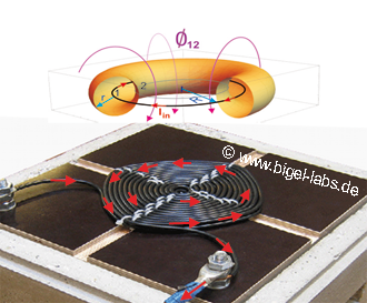
Classical electrodynamics is one of the standart lectures in universities when you study physics [1], [2]. Especially in experimental physics the concepts of induction, lenz law, lorentz force and the maxwell equations are explained via several great experiments. One of these experiments is the famous Thomson Ring Experiment (Fig. 1).
A coil with several windings creats a pulsed magnetic field by discharging a capacitor through it- or just using the alternating current from the the socket. The time dependent magnetic field induces an eddy current in a metall ring placed above the coil. The interaction of the current in the ring and the magnetic field yields to an acceleration of the ring away from the coil due the lorentz force. There are many concepts how to explain these phenomena. But no one really tells you how to calculate the currents, forces, speeds in this experiment. Physicists learn how to deal with the covariant maxwell equations, relativistic corrections, retarded potentials and fundamental concepts like the lagrangian density. In this theoretical world concepts as inductance are seen as "not to important". In engineering faculties one may hear some lectures about electromagnetic field theory- but here everything is mostly "very static" with no moving parts. With less physical background the maxwell equations are difficult to understand in any detail, so that many professors only present very easy examples to explain the electromagnetic field theory. So, as you see, the Thomson Ring Experiment is somehow between the subjects physics and electrical engineering.
In 2006 I made several studies on metal forming via pulsed magnetic fields [10]. At this time I had enough experience to do practical experiments, built high voltage capacitor banks, coils and measurement equipment. But I really had not enough mathematical and physical background knowledge to calculate a complex system as the Thomson ring experiment, which is very familiar to the electromagnetic forming technology. I remember many hollidays at my grandmas house trying to combine formulas from old austrian scool books (Schreiner) and books for electrical engineers to find a way to calculate the Thomson Ring Experiment. Everytime when I thought I got the solution I realized that I would have to know the result of an equation to use the eqution (At this time I didn´t know how to handle differential equations). This mades me very crazy and I decided to study physics. Several years later after studying physics I am proud to present a very nice concept to describe and simulate the Thomson Ring experiment here.
2. Setup of the Experiment
At this page I want to present the Thomson Ring Experiment using a capacitor as energy source (Fig. 1). After charging up the capacitor C to a certain voltage U0, the capacitor will be discharged through a flat/spiral coil. In my experiments I mostly used a 150uF capacitor bank charged up to several kV`s. While the discharge of the capacitor (here U=3kV) through the a coil with L=11uH the current reaches peak values around 12kA, which may be approximated by the formula |
|
|
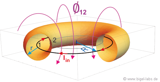
Fig. 1: Schematic setup of the Thomson ring experiment: A capacitor with capacitance C and voltage U0 is discharged through a spiral coil with inductance Lcoil. The magnetic field of the coil flushes through the Thomson ring ( Phi12) and induces an eddy current I2, which rotates in the opposite direction than the cause (rotating current I1 in the coil). The Thomson Ring then creates an own magnetic field, which is aligned contrary to the magnetic field of the coil. These two magnetic fields repel each other, so that the Thomson Ring is accelerated upwards. For an equivalent explanation with the magnetic pressure, watch my old page theory of electromagnetic forming (in German). Later I will present different concepts how to caculate the acceleration force with the lorentz force and gradient of mutual inductance (chapter 6). |
| Under (unrealistic) linear conditions with constant acceleration the acceleration path is: For a given acceleration lenght y one may solve equation [1.4] for vmax and put it into y(t) together with the acceleration time tacc [1.3]: Solving this for L we get an expression for the magnitude of inductance one should use for the coil: |
Example: |
|
| A Thomson ring with mass m=16g is accelerated by discharching a capacitor bank (U=6kV, C=150uF) through a coil. Assuming a acceleration lenght of 4cm the needed inductance of the coil is around |
||
The presented assumptions are: For practiacal experiments these assumptions are very difficult and one may have much experience and feeling to take suitable parameter values. |
Now let´s discuss the energies
in the Thomson ring experiment:
A large capacitor/capacitor bank with capacitance C is charged up to a voltage Uo [Fig. 1]. After closing the switch the energy stored in the capacitor will be transformed in the circuit. Energy conservation gives:
![]() [1.8]
[1.8]
The total energy in the system is the sum of 7 different energies:
 [1.9]
[1.9]
EC(t) is the time dependent stored energy in the capacitor, EL1(t) is the Energy of the magnetic field
in the whole circuit 1 , EM(t) is the mutual magnetic energy, EL2(t) is the magnetic energy of the cicuit 2, ER1(t) is the accumulated heat energy of the circuit 1, ER2(t) is the accumulated heat energy of the circuit 2 and Ekin(t) is the kinectic energy of the ring (circuit 2) with mass m. Before doing simulations it´s essential to know all the parameters Lcoil, Lline, Rcoil, Rline, which must be calculated before starting the simulation algorithms. Let´s first start to dicuss the calculation of the coil inductance.
3. Modelling of the coil
The coils used in the Thomson Ring Experiment are commonly in the form of Archimedean spirals. The magnetic field of such coils may be calculated with Biot-Savart law by using suitable parameterisations [12]. Practically it´s not helpful to calculate induction phenomena in metals or metal rings by using magnetic field calculations (Fig. 2b). Of course one could integrate the flux denstiy over the surrounded surface of a certain loop to get the induction current (Fig. 2b). But this requires a lot numerical effort with error propagation due to the many steps one have to follow. Remember the Poisson equation for the vector potential A: |
 |
|
| Fig. 2a: Current flow throw a spiral coil | ||
 |
||
Fig. 2b: Magnetic field flux density of a typical spiral coil with 10 windings at a current of 10kA. The magnetic flux components Bx, By and Bz were calculated via numerical integration of Biot-Savart law. The density plot shows the value Bges=sqrt(Bx^2+By^2+Bz^2). |
||
|
 [3.2]
[3.2] [3.3]
[3.3]  [3.4]
[3.4] [3.5]
[3.5] [3.6]
[3.6]The Nemann formula may be used to calculated the the self inductance Lii (with i e N) of metall rings as well as the mutual inductance Lij (i=/j) (Fig. 3).
In general one may split up the total inductance Lges of a wire into the inner inductance Lin and outer inductance Lout :
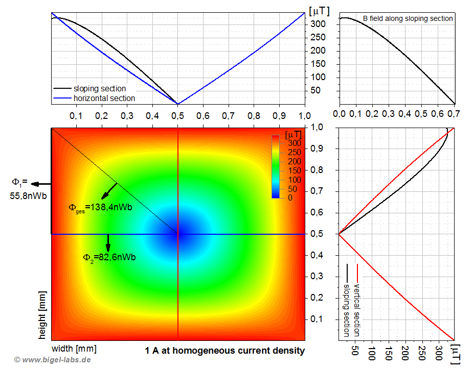
Assuming a constant partial inductance we may write and use the arithmetic expression  , [3.9] , [3.9]which may be deduced by volume integration of the energy density of an infinte long current carrying wire. For a better understanding read the excellent book from E. B. Rosa and F.W. Grover [8], [9]. The outer inductance is the inductive backlash of the conductor itself. In other words: Imagine a infinitesimal thread instead of a round wire with section A and radius r (Fig. 4). The wire has got the form of a circle with radius R. The thread carries a current Iin. Now imagine a second infinetesimal wire circle with radius R-r in the same plain. The magnetic flux (Phi12=L12*I1) through circle 2 (created by circle 1) correlates directly with the mutual inductane L12, described by the Neumann formula: |
 |
||||||
| Fig. 3: Mutual inductance between to rings: The magnetic flux created by the current I1 in ring 1 suffuses ring 2 with the flux Phi12, which is less than the flux Phi1 throw ring 1. Flux. Phi2 may be calculated with equation [3.5]. The mutual inductance L12 between the two rings is defined by the Neuman formula [3.6]. | |||||||
It is obvious, that Lout of a round wire with cross section A, radius r and circle radius R is exact L12 from the imagination with the two infinitesimal threads.
|
|||||||
The total energy of a system with several inductances and individual currents may be calculated
by integration over the energy density at each point in the space: |
|
|
Fig. 5: Model of a multilayer coil with 4 layers: Each layer has got 4 Windings as concentric circles.Via numerical simulation and comparison with real Archimedean spirals one may show that the numeric failure created by this "unreal model" is quite low for "larger winding numbers (N>10)". The radius of the smallest rings are 5mm. The radius of the other sings are 15mm, 25mm, 35mm. The distance between the three layers is 10mm. So the ring to ring distance is 10mm for any neighbor ring. The wire radius of each circle is 1mm. The inductance matrices of the coils L1, L2, L3 are the diagonal elements of the large inductance matrix below. The mual inductances between the layers are L12, L13, L23. Due the inductance matrix is symmetric L12=L21, L13=L31, L23=L32. |
 [3.15]
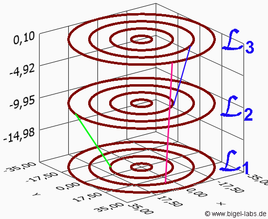
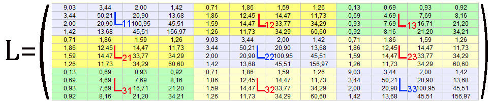
The summ of all matrix elements (equation [3.19]) is 2695nH. So the total inductance of this multilayer coil is around 2,7µH.
The explained method for inductance calculation may be used for nearly any kind of coils. You may parameterize any wire path and use the Neumann formula [3.10]. When a approximation with circles is possible, just use
equation [3.11] together with [3.13] or [3.14]. Then summarize up each element of the matrix with
equation [3.19].
3.3 Resistance of the coil - Approximation
| Since we use rings in our coil modeling the entire ohmic resistance of the coil is: The ohmic resistance of one individual ring is roughly: with the specific elctrical resistance p, which is 1,7E-2Ohm*mm^2/m for a standart copper wire. |
||
4. Selfinductance and resistance of the Thomson ring
4.1 Selfinductance
The self inductance of the Thomson ring itself is a little bit tricky to calculate. One my search in engineering books as Grover [9] or Philippow for inductance calculations of a cylindric ring [Fig. 6]. Whenever you find such a formula it´s full with strange numbers and quotients. Mostly it´s not explained how the formula is derivated. I myself do not trust such formulas without knowing the background. It´s to risky that all the simulations went wrong just because a failure in an old 100 years old formula. So the best way in my opinion is to use formula [3.13], which is absolutly derivated analytically and see how to deal with that...
Imagine a cylindric ring (Fig. 6) filled with many small filament ring circles (number n) inside. Each of the ring circles carries a current Ii=I/n. The distance between all the filament rings is constant. Then the total energy of the system is:
|
 |
|
Fig. 6: Modeling of the Thomson Ring with ring filaments inside the ring. The section of the ring is splitted up into nrad radial filaments and nh vertical filaments. The radius of each filament wire is so defined that each filament surface touches the surface of the neighbour filament. The partial inner inductance is discussed in equation [4.9]. |
For a endless round wire the partial inner inductance (watch also equation [3.9]) is
[4.8]
This inner inductance
is independent of the radius r of the wire. The inner inductance of a wire with square section (width a, height a) is a all little bit smaller than the inner inductance of a endless round wire:
![]()
 [4.9]
[4.9]
Via precise numerical field integration Iwas able to show that the inner inductance of a endles wire with square section is 48,3196 µH/m, which is around 96,6% of the partial inner inductance of a endless round wire with dL/dl=50nH/m. However for simulations I use
![]() .[4.10]
.[4.10]
| In 3.3 we approximated the wire resistance with equation [3.21], which is acceptable for the coil wire. In the Thomson ring experiment cylindric "Thomson-rings" were commonly used. According to the winding ratio of the coil to the "Thomson Ring" (one winding) and the coupling, the current flow inside the Thomson ring is mostly around ten times larger than in the coil. So here it´s better to calculate the resistance more serious. The conductance of a wire with homogenous current density is so, the differential expression depending on the radius is with the substitution dA=hdr and l(r)=2*Pi*r we get by integration over the radius r As the resistance is the inverse of the conductance, we may write 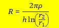 [4.14] [4.14]which is a good formula to calculate the ohmich resistance of a cylindric ring. Depending on the discharge frequency of the circuit we may also regard the skin deep of the current density in the Thomson ring. |
 |
|
Fig. 7: Thomson Ring as a cylindric ring. r1 is the inner radius, r2 is the outer radius. d ist the height of the ring. The resistance of the coil has to be calculated by integration (equation [4.13]) to regard the different circumferences. At higher frequencies the distribution of the current density is not homogen. Then it´s usefull to correct the calculated resistance from equation [4.14] due to the skin effect.
|
 skin effect calculations....
5. Mutual Inductance between Coil and Ring
5.1 Mutual Inductance via the Mutual Inductance Matrix
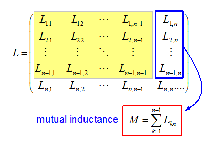
For simulations we need the value of the mutual inductance matrix for all possible heights of the Thomson ring while the acceleration. The inductance matrix of a system with n-1 circles in a flat coil and one circle with index n (Thomson ring) above the coil is:
|
 |
|
| Fig. 8: Mutual inductance components between a flat coil and a Thomson ring above the coil. The windings of the coil have got the indices 1,2,3,..., n-1. The current throw any coil circle is equal. The Thomson ring is placed above the coil with index n. The mutual inductance between the coil and the ring may be calculated with the inductance matrix shown on the left. | ||
|
||
 |
||
Fig. 9: Mutual inductance components between a flat coil with j layers and a Thomson ring above the coil. The windings of each layer of the coil have got the indices 1,2,3,..., n-1. The current throw any coil circle is equal. The Thomson ring is placed above the coil with index n. The mutual inductance between the coil and the ring may be calculated with the inductance matrix shown on the left. |
 [5.1]
[5.1]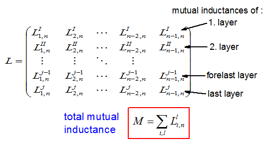 [5.2]
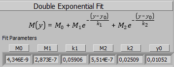
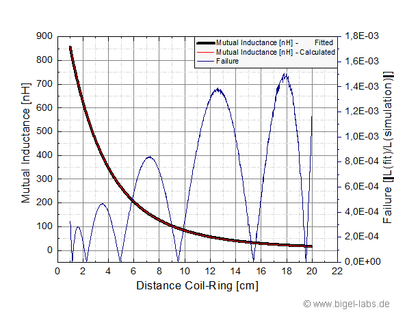
[5.2]5.2 Fitting with Multi Exponential Functions
|
6. Calculation of the acceleration force
By integration of the maxwell equation we get: [6.1] [6.1]The induction voltage is the time derivation of the total flux throw the ring. Flux Phi12 (Fig. 11) may be calculated by surface integration of the flux density Bz  [6.3] [6.3]Phi 2 is the flux created by the current I2(t) in the ring. Integration gives:  [6.4] [6.4]By this way one has to calculted first the Bz-components of the magnetic field created by the coil and the ring via Biot Savart law. Afterwards one has to integrate the magnetic field density (equation [6.3], [6.4]) numerically. Fortunately it´s easier to use the correlation between flux, inductance and currents |
|
|
Fig. 11: Eddy current induction: A time dependent current through Coil L1 creates a magnetic field, which may be calculted by Biot Savart law. A certain part of the total flux Phi12 flushes throw the Thomson ring above the coil. This flux may be calculated via surface integration of the magentic flux density in the ring plane (equation [6.3]) or just by using the mutual inductance expression (equation 6.5). |
| Using equation [6.2] we may write directly The mutual inductance L12=M varies by time, so that we get the expression With Ohm´s law we get for the current The Lorentz force Fz(t) created by the current I2(t) then is As shown in Fig. 12 only the Bz-components in the ring plain are responsible for the induced current I2. |
|
|
Fig. 12: Lorentz force Fz: The Lorentz force on the Thomson ring depends on the radial magnetic field Br inside the ring and the current flow inside the ring I2. The current flow I2 depends on the changing of the Bz- components of the magnetic field created by the coil. |
The Br-components inside the ring are responsible for the Lorentz force (equation [6.9]). So, finally the lorentz force depends on a very tricky relation of the Br- and Bz-components.
6.2 Via Gradient of mutual inductance
Another moore practical method to calculate the acceleration force is to use the gradient of the mutual inductance.
The total magnetic energy of the system is:
Mechanical variation of the magnetic energy gives the differential expression Differentiation to the height y yields: The corresponding force to the potential E is described by the gradient [1], [2]: Therefore the acceleration force in z-direction is: With the double exponential function (equation [5.2]) we may easily write the expression |
|
|
Fig. 13: Coherence between the gradient of mutual Inductance and force: Fz is proportional to the currents I1, I2 and the gradient of mutual inductance between the ring and the coil. With this method there is no need to calculate the magnetic field components Bz, integrate over the flux density and calculte Br. |
which is very usefull to calculate the acceleration force (Fig. 13).
6.3 Table of Differential Equations
After discussing all the inductance theory and force calculations we are now ready to deduce all differential equations needed for numerical simulations.
With Kirchhoff´s voltage law we may write for the first circuit:
![]() [6.16]
[6.16]
Neglecting the line inductance Lline we may set L1=Lcoil (remember Fig. 1). Then the the Voltage UL1(t) is equal to the changing of the magnetic flux through the circuit:
![]() [6.17]
[6.17]
The magnetic flux
through the first circuit is the flux created by the inductance L1 and the flux created by the inductance L2. So we may write
![]() [6.18]
[6.18]
Differentiation gives
![]() , [6.19]
, [6.19]
while dL1/dt=0. Solving the equation to dI1/dt gives:
![]() [6.20]
[6.20]
With Kirchhoff's second law the second circuit
gives:
![]() [6.21]
[6.21]
Differentiation to time yields
![]() .[6.22]
.[6.22]
![]() [6.23]
[6.23]
So finally we get:
![]() [6.24]
[6.24]
Solving to dI2(t)/dt gives:
![]() [6.25]
[6.25]
Putting dI1(t)/dt into dI2(t)/dt gives:
![]() [6.26]
[6.26]
After solving
dI2(t)/dt we get:
![]() [6.27]
[6.27]
For
dI1(t)/dt we get:
![]() [6.28]
[6.28]
The Voltage on the capacitor Uc(t) may be described by
|
||
Maybe you miss a minus, because the force is a negative Gradient. Since the currents I1(t) and I2(t) are rotating in opposite directions (watch Fig. 17 later) and our quotation in equ. [6.34 ] the product I1(t)*I2(t) is negative for 0<t<1/3Pi*sqrt(LC), which is the main accelleration time intervall. With dM(y(t))/dt<0 for every time we get a positive force in y-direction with expression [6.35]. Substitution of dM(y(t))/dt gives the formula for the acceleration of the ring in y-direction:
![]() [6.36]
[6.36]
Now we may put all found expressions in one table of differential equations:
| Nr. | Boundary Conditions |
Differential Equation | solved function |
| 0 | I1(0)=0 | I1(t) | |
| 1 | I2(0)=0 | I2(t) | |
| 2 | Uc(0)=Uo | Uc(t) | |
| 3 | y(0)=0 | y(t) | |
| 4 | v(0)=0 | v(t) | |
| 5 | E1(0)=0 | E1(t) | |
| 6 | E2(0)=0 | E2(t) | |
| 7 | A(0)=0 | A(t) | |
Before solving the differential equations the functions M(y(t)) and dM(y(t))/dt must be substituted with:
| |||
These 8 differential equations may be solved numerical using Runge Kutta Algorithms. I prefer using adaptive step size regulation methods as the Cash Karp algorithm. By using this method I built a graphical used interface programm, which is great for realistic simulations of the Thomson ring experiment.
7. Simulation of realistic experiments
7.1 Software
The simulation software I built contains a front panel where all relevant data (Capacitor Bank Data, Spiral Coil Data, Algorithm Parameters) may be putted in (Fig. 14). After putting in all needed data the inductance of the Thomson ring is calculated first by using the method described in chapter 4.1.
Fig. 14: Front Panel of the Simulation Software: In the top all needed data may be entered. The Thomson ring inductance is approximated by n ring filaments depending on the Filament-density.
In a next step the programm calculates the mutual inductance between the Thomson ring and the coil by using the method from chapter 5. The mutual inductance curve is fitted by a double exponential function automatically (Fig. 15).
 Fig. 15: Mutual Inductance Fit: Fit tolerance and mumber of iterations may be adapt to the dimensions of a specific experimental setup. On the right side a work coil (here one layer) and the Thomson ring above is shown.
The inductance matrix of the work coil is calculted by the methods presented in chapter 3.2. It´s possible to define a work coil with several layers for higher inductances. Summation over all ring resistances of the work coil gives the total resistance of the coil (chapter 4.2). All these data are used in the software to substitute the parameters of the differential equations. Numerical solving of the differential equation system via Runge Kutta Algorithms enables the software to show many interesting graphs (Fig. 16):
 Fig. 16: Simulation results 1: a) voltage and current at the capacitor b) Sum of all energies c) Height force Graph d) position height of the ring e) speed of the ring f) kinetic energy of the ring
The discharge current of the electrical circle may be compared with the induced current in the ring in one graph (Fig. 17a). The Action integral value may be analysed as a function of the time (Fig. 17b) to reduce over current damaging effects of the used capacitor.
Fig. 17: Simulation results 2: a) current in the ring (plot 0) and discharge current (plot1) b) Action Integral curve
Futher the magnetic energies (Fig. 18a), capacitor energy (Fig. 18b), mutual inductance energy (Fig. 18c) are plotted. Together with the total heat energy in the discharge circle (Fig. 18d), the heat energy in the Thomson ring (Fig. 18e), the sum of all energies (remember equation [1.9]) of the system is presented (Fig. 18f). With this graph the energy deviation from the start energy may be analysed to get a feeling how accure the simulation works. In the presented example the maximal deviation is only appr. 0,6mJ, which is really small compared to the total energy of 1200J.
Fig. 18: Simulation results 3: a) magnetic energy of inductance L1, L2 b) capacitor energy c) mutual inductance energy d) heat energy e) heat energy in the ring f) sum of all energies
Comparing al the plotted energies one may easily find some parameters wich may be improved to get a higher efficiency. In the next chapter I want to compare three different flat coils to find out the specific differences.
7.2 KB1-KB2-FL1,2,3 Experiment Simulations
While the project Metallverformung durch Kurzpulsmagnetfelder 2006 I developed a set of different flat coils with an inductance of 11uH, 45uH and 100uH. Assuming a Aluminium ring with r1=50mm, r2=53mm, h=6mm one may simulate a pulse discharge of the capacitor bank KB1-KB2 to accelerate the Thomson Ring. Calculation of the standart resonance frequency and taking the skin effect into acount the following table of data is obtained:
used Coil |
measured coil inductance |
calculated coil inductance |
standart frequency f0 |
Thomson ring resistance correction |
FL1 |
11uH |
11,1uH |
3240 Hz |
116% |
FL2 |
45uH |
42,3uH |
1890 Hz |
105% |
FL3 |
100uH |
91,0uH |
1330 Hz |
103% |
Due to the skin effect I used a correction of the electrical resistance depending on the standart resonance frequency. By simulation of these experimental setups I got the following results:
 |
 |
| Fig. 19a: Height of the Thomson ring: With the FL1-Setup the acceleration of the ring is the highest within the first 100us. Anyway with the FL2-Setup one gets the fastest gain of height. | Fig. 19b: Speed of the Thomson ring: The final speed of the ring with FL2 is 129,2 m/s. With the FL3-Setup the maximal speed is 109,8m/s compared to the FL1-Setup with 109,8m/s. The end speed is achieved at around 1ms. |
The acceleration of the Thomson ring with the FL1-Setup is the highest in the first 100us (fig. 19a). After 200us the speed of the ring in the FL1 experiment is much less than in the other experiments (Fig. 19b). After 1ms there is no moore significant acceleration. It´s obvious that the highest ring speed may be achieved with the FL2 experiment. In my old experiments I also got the best electromagnetic forming results by using the FL2-coil. The discharge current flowing throw the coils has got a absolute maximum of appr. 12,8kA in the Fl1 experiment, compared to 7,1kA with the FL2 and around 5kA with the FL3 experiment (Fig. 20a). The induced current in the ring is much higher than the discharge current flowing throw the coils (Fig. 20b). Surprisingly the maxima of the ring currents are quite similar between 40kA´s and 45kA´s.
 |
 |
| Fig. 20a: Discharge current of the circuit. | Fig. 20b: Induced current in the Thomson ring: The current maximum in the ring is very similar for the FL1 and FL2-Setup with around 45kA. |
Capacitor voltage curves are important because the reversal voltage is the main damaging factor reducing the life time of high voltage capacitors. In the simulations the reversal voltage is between -3,0kV and -3,5kV (Fig. 21a). This indicates a low damping of the circuit enery oszillation. Numerical solving of the the differential equations number 5 and 6 (table in chapter 6.3) the absorbed heat energy in the circuit (R1) and the ring (R2) may be calculted. The results are plotted in Fig 21b. The heat energy in the ring is quite similar for all used coils (dotted lines in Fig 21b). This means that the numerical value of the action integral A(t) of the ring current is similar for any used coil. The absorbed heat energy in the circuit is mainly affected by the Action Integral, whose value compensates the small resistance of the FL1 coil compared to the other coils. This strange effect yields to a fast heating of the FL1 coil (blue line FL1-heat R1 in Fig. 21b), although this coil has got the lowest restistance. The heat absorbtion curves of the FL2 and FL3 coils are significant less rising.
 |
 |
| Fig. 21a: Voltage curves | Fig. 21b: Heat energies |
| Nevertheless for long times the absorbed energy in the circuit is quite similar for all investigated experiments. The absorbed circuit heat energy in the FL1-experiment is 80,1% of the start energy, compared to 76,6% in the FL3 and 76,2% in the FL2 experiment (Fig. 22). The total ring heat energy is around 12-13% in the experiments. With the FL2 experiment one may get the best mechanic efficieny, so that the kinetic energy of the ring reaches 10,9% of the start energy. The kinetic energy of the Thomson ring in the FL3 experiment is 10,7% followed by 7,9% in the FL1 experiment. So the efficiency of acceleration is around 10% of the start energy in in the capacitor for all investigated experiments using the coils FL1, FL2 and FL3. |
 |
| Fig. 22: Final Energy distribution of the Thomson ring experiment |
With a self built software the evaluation of simualtion results gives now the opportunity to improve practical experiments. The suitability of the built software could be tested by the simulation of the Thomson ring experiment with my coils FL1, FL2 and FL3 and the capacitor bank KB1-KB2 as energy source. Analysis of the simulations gave a maximum acceleration efficiency of around 10% with the used Thomson ring. The graphs of ring position, speed, voltage, currents, heat energies may be obtained and analyzed to understand the differences.
In further practical experiments these results should be validated by measurements. This could lead to a even better adjustment of the simulation parameters as skin effect corrections and sparc gap resistance influence. In a next project I will analyse the eddy current density and pressure distribution of larger metal sheets instead of using a Thomson ring....
[1] Introduction to Electrodynamics, Addison Wesley; 3rd edition, David J. Griffiths
[2] Classical Electrodynamics, John David Jackson
[3] Simulation and verification of Thomson actuator systems, Ara Bissal, Göran Engdahl, Ener Salinas, Magnus Öhström, COMSOL Conference Paris 2010
[4] HIGH-SPEED AC CIRCUIT BREAKER AND HIGH-SPEED OCR, Young-woo JEONG, Hyun-wook LEE, 22nd International Conference on Electricity Distribution
[5] Shape Optimization of a Thomson Coil Actuator for Fast Response Using Topology Modification, Wei Li and Chang Seop Koh, Journal of Electrical Engineering & Technology Vol. 7, No. 1, pp. 58~63, 2012
[6] Optimizing Thomson’s jumping ring, Paul J. H. Tjossem and Elizabeth C. Brost, Department of Physics, Grinnell College, Grinnell, Iowa 50112
[7] Klassische Mechnik, F. Kuypers, Wiley-VCH, 5.überarbeitete Auflage
[8] Formulas and Tables for the Calculation of Mutual and Self Inductance, E. B. Rosa, F.W. Grover, U.S. Dept. of Commerce and Labor, Bureau of Standards : 1912
[9] Inductance Calculations, F.W. Grover, Dover Books on Electrical Engineering, 1 edition, 2009
[10] Metallverformung durch Kurzpulsmagnetfelder, Max Bigelmayr, Jugend forscht Projekt 2006
[11] Discharge behavior of capacitor banks, Max Bigelmayr, 2011
[12] Berechnung der Magnetfelder von Spulen, Max Bigelmayr, 2010
Last update: May 2015, August 2015 (V1)